
An Analysis of “Graham’s Net-Nets: Outdated or Outstanding?”
- Gaurang Merani

- Oct 8, 2019
- 5 min read
Updated: Aug 1, 2020
Introduction
In an earlier post we analyzed the prominent and often cited study on “net nets”, “Benjamin Graham’s Net Current Asset Values: A Performance Update”, conducted by Henry R. Oppenheimer from the Financial Analysts Journal (1986). In this post we analyze the article “Graham’s Net-Nets: Outdated or Outstanding?” by James Montier. The objective of the article was to examine the performance of securities that were trading at no more than two-thirds of their “net current assets” during the 23 year period from 1985-2007 globally and regionally (namely, in the US, Europe and Japan(i)).
Our objective was to analyse the article itself; determine its reliability, draw our own conclusions and glean, if any, actionable advice for the practitioner of the “net net” method of investing.
Summary
We simply replicate the summary provided by the author for ease of reference before conducting our own analysis.
Value Investing: Tools and Techniques for Intelligent Investment, Chapter 22, p. 230/231:


Key Methodology
Valuation metric: “…current assets minus its total liabilities…”
The author did not expressly state whether preference shares were also deducted from Current Assets; however, we assume the formula used was as specified by Graham:
i.e. Net Current Asset Value per share = (Current Assets – (Total Liabilities + Preferred Shares))/Common Shares Outstanding
“Of course, Graham wasn’t contented with just buying firms trading on prices less than net current asset value. He required an even greater margin of safety. He would exhort buying stocks with prices of less than two-thirds of net current asset value (further increasing his margin of safety). This is the definition we operationalize below.” i.e. the study examines the returns to stocks trading at less than 2/3 of net current asset value.
Weighting: “equally weighted”
Purchase/rebalance date: unspecified
Holding/rebalancing period: unspecified
Reliability
While there are numerous biases/errors that can be made when conducting studies/back tests, below we have analysed those we deem most likely to impact a study of this nature:
1. Survivorship bias
Given the data source was not specified and no mention was made of controlling for survivorship bias we have no way of knowing if the sample studied may have suffered from survivorship bias.
2. Look Ahead bias
No mention was made with regard to the portfolio formation date, so we do not know if the back test suffered from Look Ahead bias, or not.
3. Time period bias
The study spans 23 years and we classify this as a “more reliable” period.
For reference:
< 10 years; inadequate/unreliable
11 to 20 years; somewhat reliable
> 20 years; more reliable
> 40 years; most reliable
4. Human error
Human error is always a possibility; however, we have little detail on the back-testing protocol implemented so cannot comment on the increased or decreased likelihood of human error entering the testing process.
5. Journal rating/credibility(ii)
Given this was essentially an article we cannot assign it with the additional credibility afforded to publications appearing in well renowned finance journals.
Reliability Assessment: Given the absence of detail pertaining to the methodology and data source used to undertake the back test we deem the article to possess a low level of reliability. In addition, further analysis (refer below) causes us to question the reliability of the results generally.
Results and Analysis
“An equally weighted basket of net-nets generated an average return above 35% p.a. versus a market return of 17% p.a.”
“Not only does a net-net strategy work at the global level, but it also works within regions (albeit to varying degrees). For instance, net-nets outperformed the market by 18%, 15%, and 6% in the USA, Japan and Europe, respectively.”


We summarise the results in the table below (some of which were gleaned from Figure 22.2):
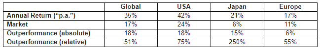
The author specified that the returns were “p.a.” i.e. per annum. It is not clear, to us, if “p.a.” represents the arithmetic mean or geometric mean i.e. the compound annual growth rate. This, in our opinion is of critical importance, especially given the length of the study and given it incorporated Japan, a market which experienced, to our knowledge, the greatest stock market bubble in recorded history during the period examined. But how could we find out?
Interestingly the author refers to the Oppenheimer study with which we are intimately familiar.
“In 1986, Henry Oppenheimer published a paper in the Financial Analysts Journal examining the returns on buying stocks at or below 66% of their net current asset value during the period 1970–1983. The holding period was one year. Over its life, the portfolio contained a minimum of 18 stocks and a maximum of 89 stocks. The mean return from the strategy was 29% p.a. against a market return of 11.5% p.a.”
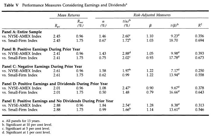
Table V from the Oppenheimer study is reproduced below for ease of reference:

Using the above information, we can deduce the following with reasonable confidence:
The author derived “29%” by multiplying the monthly portfolio return of 2.45% by 12 i.e. 2.45% * 12 = 29.4% i.e. “29%”.
The author derived “11.5%” by multiplying the monthly market return of 0.96% by 12 i.e. 0.96% * 12 = 11.52% i.e. “11.5%”.
We know the compound annual growth rate in the Oppenheimer study for the full sample period was 28.2% (refer table IV, not reproduced here). Compounding 2.45% for 12 months yields 33.7% ((1+ 2.45%)^12-1). Therefore, we determine that the results in table V of the Oppenheimer study represent the arithmetic mean and not the geometric mean referred to in Table IV. Hence, based on the comparative statistics referenced by the author, we deduce, with a strong likelihood, that the author has calculated the arithmetic mean return.
The implication of calculating the arithmetic mean return vs the geometric mean return is stark. The arithmetic mean would, on the balance of probability, have materially overstated returns. Of particular concern are the returns stipulated for Japan which experienced, to our knowledge, the largest equity market bubble in recorded history in the late 1980’s which formed part of the period studied (i.e. 1985 to 2007). To illustrate the misleading nature of an arithmetic mean we refer to the “Summary Edition Credit Suisse Global Investment Returns Yearbook 2019” Table 1:

There is a material difference between the arithmetic and geometric mean achieved for all equity markets examined. For Japan the arithmetic mean is more than double the geometric mean! While the returns quoted are “real” returns and the time period different, our point remains, an arithmetic mean has, and does, overstate the actual returns achieved.
Moreover, a cursory glance at Figure 22.2 illustrates returns of 24% p.a. to the “USA Market” from 1985-2007; this also indicates an arithmetic mean has been used because, to our knowledge, the US market simply did not achieve a compound annual growth rate of 24% from 1985 to 2007!
To take our point to a theoretical extreme let’s examine a short series of returns calculating both the arithmetic and geometric mean:


Remarkably, it is theoretically possible to achieve an arithmetic mean twice that of the market (16.00% vs 8.00%; 2x); and simultaneously attain only a fraction of that return based on the geometric mean (4.99% vs 0.95%; 0.19x).
Conclusions and Practical Implementation
Given the relative dearth of studies examining the returns of net nets, especially those in Japan, we are grateful for this article. Nonetheless, due to the silence on the data source, details pertaining to the research methodology and the strong likelihood that the returns specified were calculated using the arithmetic mean, thus overstating returns, little can be relied on from this article.
While it may be disheartening to be left with something of a “null hypothesis”, it does provide us with the opportunity to be clichéd and conclude with a quote from none other than Charles T. Munger:
“Any year that passes in which you don’t destroy one of your best loved ideas is a wasted year.”
Notes:
(i) Please note, the article did not state which exchanges were examined in the markets studied.
This article was also published by Alpha Architect here


Comments